In previous blogs we have already introduced this problem and some of the typical ways to solve it. This time we are going to introduce new resolution methods and expand the comparison we made previously to take these new methods into account.
1.- Method 2-opt and 3-opt
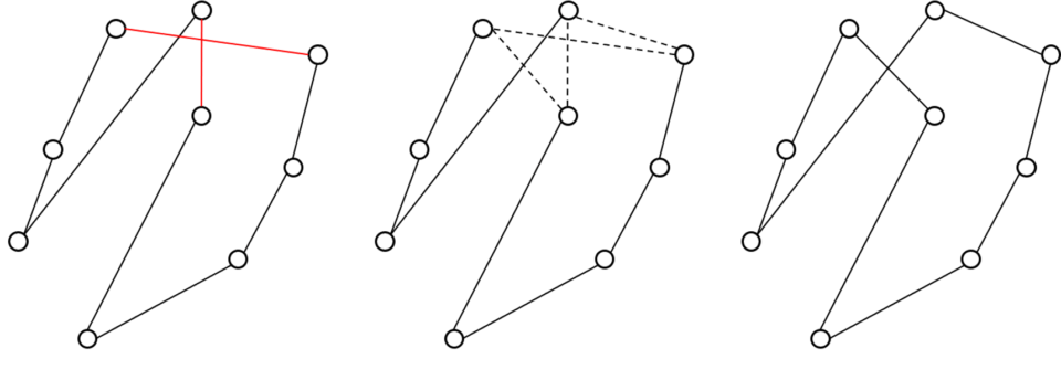
Both methods are simple TSP problem-specific local lookup methods. The 2-opt method was proposed in 1958 by Croes. This method consists of selecting two arcs of the complete graph, eliminating them and evaluating the other reconnection position of the graph that allows obtaining a lower cost. An example of this process can be seen in the following image:
Figure 1. Example 2-opt method.
The red arcs are the ones that are studied here, first they are eliminated and a selection is made between the existing one and the new one (according to which one represents the best connection).
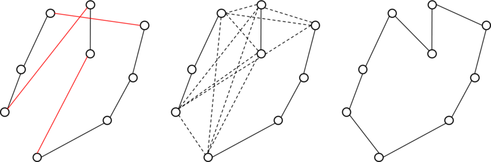
The 3-opt method is an extension of the previous one, but in this case 3 arcs are eliminated and the connections that do not generate sub-cycles are evaluated. Again in the following figure you can see an example.
Figura 2. Ejemplo aplicación método 3-opt.
In this case we can see that by applying a 3-opt change we are able to find a better solution from the same starting point as with the 2-opt change.
As a general rule, the 3-opt method is slower, its complexity is O(n^3), than the 2-opt method, but it usually generates better solutions.
2.- Simulated annealing
In this case, simulated annealing is a metaheuristic technique to approximate the global maximum or minimum of a function. In this case we use simulated annealing combined with the 2-opt and 3-opt techniques.
Simulated annealing is inspired by the annealing process in metallurgy and consists of establishing a temperature, which is reduced as the iterations of the method pass. This temperature is used to regulate the acceptance of changes in the problem that do not imply a better solution, in such a way that the higher the temperature, the greater the probability of accepting a “worse” solution.
This process allows a better exploration of the solution space and therefore a better solution can be found.
In our case, if when evaluating a configuration with the 2-opt or 3-opt we obtain a value solution compared to the initial one, in the normal methods we would only accept them if , c0>c1, but in the simulated annealing changes are introduced in this process:
First you get a random number between 0 and 1.
If the temperature is greater than that number and the change is accepted.
Otherwise, the iterations continue.
3.- Comparison
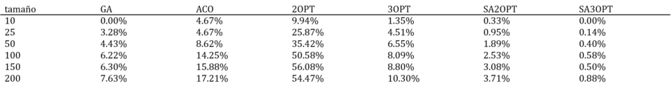
To carry out the comparison of these methods we have generated 10 examples for problems of 10, 25, 50, 100, 150 and 200. The results presented are therefore the means for each problem size.
In addition, in this case we also included the DFJ formulation presented in the previous article to compare its results. In the case of the integer models, the SCIP solver has been used since it has recently released its use.
Therefore, the models to compare are:
Whole model DFJ (DFJ).
Genetic algorithm (GA).
Ant colony (ACO).
2-opt (2OPT).
3-opt (3OPT).
2-opt simulated annealing (SA2OPT).
3-opt simulated annealing (SA3OPT).
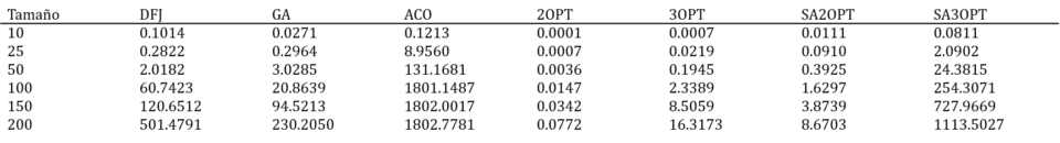
In the first table you can see the deviation for each method compared to the best (DFJ), while in the second you can see the average time, in seconds, necessary to reach said solutions for each one of the methods. It is worth noting that for instances with 200 nodes, the exact method (DFJ) has not been able to obtain a solution, so the comparison is made with 9 instances.
Table 1. Comparison method.
It is possible to verify some methods are very close to obtaining the local optimum even in large instance sizes. As in the previous blog, the results of the genetic algorithm are very good, while in this case the ACO has suffered worse results by limiting the execution time to obtain solutions.
The new methods present different qualities of results, while the 2OPT is the worst of all, which was expected, given its deterministic nature and its limitation when making changes. The 3OPT presents better results and close to those of the genetic algorithm.
Finally, the version of these two methods with simulated annealing is considerably improved and in the case of SA3OPT the best results of any method are obtained.
Table 2. Comparison method.
As shown in the time table, many of the heuristic and metaheuristic methods are capable of finding solutions in less time, with the exception of ACO and SA3OPT. In the first case , it is due to the high computational complexity of some of the necessary calculations of the metaheuristic, while, in the case of the SA3OPT, given the high number of possible combinations and the simulated annealing process, its execution time be so high
Given the results and the average execution times, it is possible that in certain circumstances it is of great interest to use one of the heuristic or metaheuristic techniques.
If you like solving problems like this, baobab is your place, check out our job offers, and if you’re curious to see how these problems have been solved, hereyou have all the code.
REFERENCES
Croes, G. A. (1958). A method for solving traveling-salesman problems. Operations research, 6(6), 791-812.