
The travelling salesman problem
The travelling salesman problem (TSP) consists on finding the shortest single path that, given a list of cities and distances between them, visits all the cities only once and returns to the origin city.
Its origin is unclear. A German handbook for the travelling salesman from 1832 mentions the problem and includes example tours across Germany and Switzerland, but it does not cover its mathematics.
The first mathematical formulation was done in the 1800s by W.R. Hamilton and Thomas Kirkman. Hamilton’s icosian game was a recreational puzzle based on finding a Hamiltonian cycle, which is actually a solution to the TSP problem in a graph.
The TSP can be formulated as an integer linear program. Although several formulations are known to solve this problem, two of them are the most prominent: the one proposed by Miller, Tucker and Zemlin, and the one proposed by Dantzig, Fulkerson and Johnson.
These methods can theoretically return an optimal solution to the problem but as this is considered an NP-hard problem, they can be too expensive both in computation power and time.
In order to obtain good solutions in a shorter time, a lot of effort has been made to try and solve this problem with a variety of heuristic methods. Out of this whole group of heuristics, we would like to highlight those inspired in biology: Ant Colony Optimization (ACO, which we talked about before here) and Genetic Algorithms (GA).
Integer Linear programme
As we mentioned there are two main formulations for the TSP, the proposed Miller, Tucker and Zemlin (MTZ) and the Dantzig, Fulkerson and Johnson (DFJ). Although the DFJ formulation is stronger, the MTZ formulation can be useful.
MTZ formulation
The mathematical formulation proposed by Miller, Tucker and Zemlin is as follows:
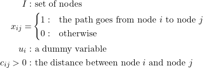
Using this set, the two variables and the parameter we can then formulate the problem as:
![\[min \sum_{i=1}^{n}\sum_{j\neq i,j=1}^{n}c_{ij}x_{ij}\]](https://baobabsoluciones.es/wp-content/ql-cache/quicklatex.com-889a4bf6b9925d0d79a80181d5acf5cf_l3.png "Rendered by QuickLaTeX.com")
Subject to:
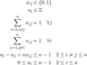
The first and second equations enforce the type of the different variables, the third and fourth equations ensure that each node is reached and departed only once, while the last two equations enforce that only one route crosses all the nodes.
DFJ formulation
In the formulation proposed by Dantzig, Fulkerson and Johnson we begin with the same variable  and parameter
  so that he formulation can be completed with:
![\[min \sum_{i=1}^{n} \sum_{j \neq i, j=1}^{n} c_{ij}x_{ij}\]](https://baobabsoluciones.es/wp-content/ql-cache/quicklatex.com-6fbb1a77a284dd77896d330585863d26_l3.png "Rendered by QuickLaTeX.com")
Subject to:
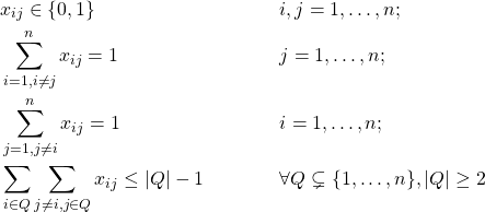
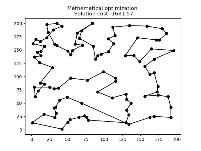
The first three equations are the same as in the previous formulation, and the new constraint (last one) ensures that there are no sub-tours, so that the solution returned is a single tour and not the combination of smaller tours. Because this leads to an exponential number of possible constraints, in practice it is solved with delayed column generation.
In the following graph we can see the optimal solution for a 100-node problem.
Ant colony optimization
Also known as Ant Colony System (ACS) or Ant System (AS), it is a probabilistic technique or heuristic used to solve problems that can be reduced to finding good paths in graphs. This method was initially proposed by Marco Dorigo in 1992 in his PhD thesis.
In the following animation it can be seen how this heuristic works for a problem and evolves improving the solution over time.
In the animation the red shadows represent the amount of pheromones deposited by the ants during the calculations.
Do you want to stay up to date with blogs like this? Subscribe to our Newsletter.

Genetic algorithm
Genetic algorithms (GA) are heuristics inspired by the evolution process of living things. Each solution is a chromosome composed by genes which represent the different values of the variables of the solution.
Starting with an initial population, we can make the solutions “evolve” over iterations. The process consists in selecting the best half of the population from which we randomly pick pairs of chromosomes (solutions) for mating. In these mating we interchange genes from both solutions to generate new solutions (children).
After the mating process we randomly apply mutations in the resulting children in order to further explore the solution space.
Finally we select the best 50 individuals from the population (the initial plus the children) and continue the process until we converge into a solution.
In the following animation we can see how the genetic algorithm evolves for the same 100-point problem.
Comparison
As it can be seen in the graphs above each heuristic provides a solution to the problem, although some better than others. When we test these three methods in more datasets we can find the following results:
| LP | LP | ACO | ACO | GA | GA | |
|---|---|---|---|---|---|---|
| Nodes | Perf. | Time | Perf. | Time | Perf. | Time |
| 5 | – | 0.06s | – | 0.04s | – | 0.08s |
| 10 | – | 0.17s | 3.22% | 0.2s | – | 0.1s |
| 25 | – | 0.72s | 23.68% | 1.09s | 28.94% | 0.17s |
| 50 | – | 1.75s | 26.42% | 4.04s | 66.04% | 0.24s |
| 75 | – | 3.04s | 14.67% | 11.61s | 84.00% | 0.33s |
| 100 | – | 6.43s | 11% | 16.32s | 96.00% | 0.44s |
| 150 | – | 16.73s | 6.67% | 180.69s | 70.00% | 2.78s |
| 200 | – | 56.17s | 5.00% | 267.42s | 92.50% | 3.47s |
| 250 | – | 252.06s | 3.60% | 503.31s | 90.80% | 7.58s |
The performance is calculated as the deviation between the solution provided by each method and the best solution found for that instance.
In very small instances all methods reach the same solution but as the instances get bigger the heuristics start to deviate from the best solution found by the integer linear programme. Although the genetic algorithm shows a larger deviation from the optimal solution, it can still provide a solution within a shorter time than the other methods. Probably, if we were to increase the population in order to better explore the solution space we could get better results without sacrificing processing time.
ACO is the heuristic (and the one exclusively devised for this problem) that can keep with the exact model, but it takes longer to arrive at a solution.
To solve the integer linear model we need a mathematical solver, which can be either free or commercial. For this post we used a commercial solver that actually improves the performance exponentially in contrast to the free ones. This advantage is what makes the integer linear problem faster than ACO. If we were to try free software, ACO would provide better solutions in a shorter time, using an open-source language (python).
If you like solving problems like this, baobab is your place. Check out our job offers.
Check here how these algorithms to solve the Travelling Salesman Problem are developed with python.
By Guillermo González-Santander, Project Manager at baobab.