
One of the most important challenges that Energy Trading departments face is how to deal with uncertainty regarding purchase and sale decisions. In this post we will explain, with a very simple example, what it entails to optimize these decisions in uncertain volatile markets, where predictions are not sufficiently reliable.
We will begin this example using deterministic techniques and then we will apply stochastic techniques that specifically deal with uncertainty. These techniques are applicable to trading decisions for electricity, gas, hydrocarbons or other raw materials.
Deterministic linear optimization example
In order to simplify this example, we will assume that the trader has to make decisions to sell raw material in tons. In general terms it could have referred to the purchase of electricity in MWh. In addition:
- We will focus on the surpluses of a single raw material during a specific month.
- We have a fixed amount to sell during said month.
- We operate in two markets where we can sell that surplus.
- Each market has a different selling price and market conditions.
The goal is to determine the optimal decision with a given set of constraints:
- There is 20,000 tons of some raw material to be sold in a month.
- In market 1, we have a closed contract with a minimum quantity of 6,000 t at 1 c.u./ t.
- In market 2, a maximum of 15,000 tonnes can be bought and the selling price is 1.5 c.u./ t.
The first step to find the optimal solution is to formulate the problem:
- Decision variables – Xi: t to be sold in each market, where i is 1 or 2 (market 1 or market 2)
- Objective function – Max Z = 1 · X1 + 1.5 · X2
- Constraints:
- X1 ≥ 6.000
- X2≤ 15.000
- X1 + X2 ≤ 20.000
- X1,X2≥0
As this case is limited to two markets, it is possible to find the optimal solution by representing the constraints and the objective function on a graph with two axes corresponding to each market:
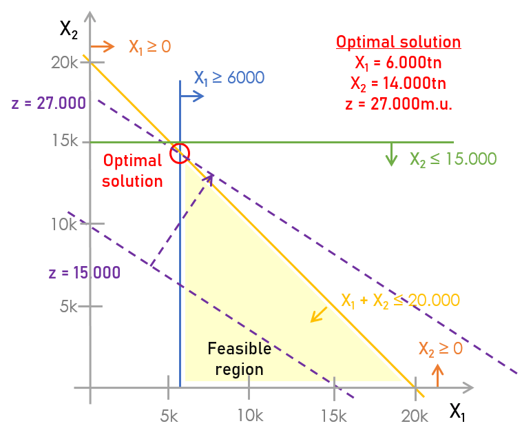
The optimal decision is, among all the possible ones, to sell 6,000 t in market #1 and 14,000 t in market #2, obtaining for this sale a total of 27,000 monetary units (€, $ or whatever currency is used).
Real-life problems are usually much more complex, with more raw materials and surpluses to be sold, more months to be simultaneously evaluated, with a daily decision window or more sale restrictions in each market.
In relation to this aspect, the problem can be complicated further when, for example, constraints include a minimum quantity per contract for a set of months and a minimum quantity per month, monthly quantities in multiples of a quantity corresponding to container capacity or markets where price depends on raw material quality or sales volumes.
Ultimately, finding the optimal solution in real trading environments is not trivial, and it is required to use Prescriptive Analytics techniques to make sure that the decision is not only good, but that it is mathematically optimal. Traders who make optimal decisions obtain higher margins than those who make good decisions.
Linear optimization under uncertainty
But the real optimization problem is even more complex. What if we take uncertainty into account?
Let’s take a look:
In the absence of uncertainty, all the parameters (ci = coefficients that multiply the decision variables in the objective function, aij= coefficients that multiply the decision variables in the constraints, and bj = coefficients that appear at the extreme right of the constraints) know each other with certainty.
However, if we take uncertainty into account, one or more model parameters are not known with certainty, but its probability distribution or a set of possible scenarios are known.
There are different approaches to dealing with uncertainty:
- Stochastic optimization. Given a set of scenarios (values of the uncertainty parameters and associated probabilities), we want to obtain a feasible solution that maximizes the expected benefit or minimizes the expected costs for the whole set.
- Chance constraints optimization. This case is a variant of the previous one, where some of the model’s restrictions are satisfied with a certain probability. For example, if a chance constraint has a probability of 95%, this means that the constraint must be satisfied for (at least) 95% of the analysed scenarios. This approach can be used to assign less weight to less frequent scenarios.
- Robust optimization. Given an uncertainty set in which the uncertainty parameters can move (box or ellipse format, for example), we aim to design feasible, close to the optimum, solutions. This is recommended when feasibility is considered more important than optimality.
Stochastic optimization
Let’s study a more complex variant of the previous problem using stochastic optimization.
In particular, we will assume different product pricing scenarios. This is the most basic case, which allows to illustrate the essence of stochastic optimization. However, there are more complex and much more powerful variants. For example, there may be different demand scenarios or we can even consider purchases for different periods and the different price and demand scenarios in each of them (multi-stage models).
- Same amount of surplus.
- Three markets:
- Market #1. Now, we can decide whether or not to sell in this market, but if we decide to sell, we must sell at least 6,000 t.
- Market #2. Same conditions as before, only a maximum of 15,000t can be sold.
- Market #3. New market without minimum or maximum sale limits.
- Three price scenarios each with an associated probability (0.2, 0.4 and 0.2, respectively). In this case, stochasticity is on ci (= sell price).
This problem can no longer be solved graphically because it contains more than two variables.
Deterministic vs. Stochastic model
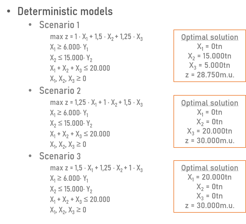
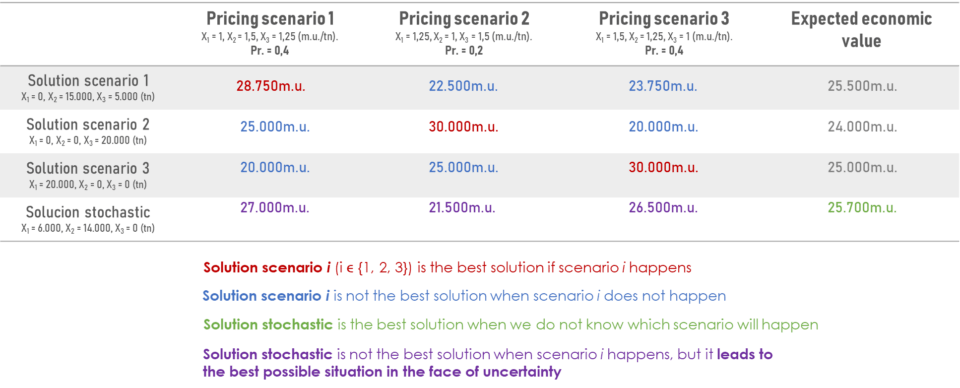
Deterministic model. This model is used to evaluate each scenario independently. As a result, there are three solutions: the best solution for each of the deterministic scenarios.
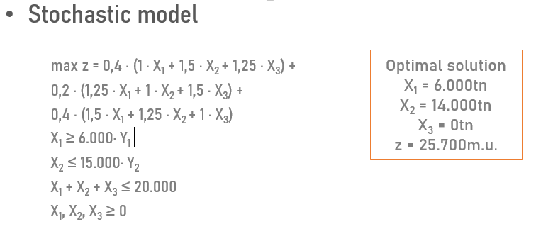
Stochastic model. This model is used to evaluate all three scenarios combined. As a result, there is a single solution for all three scenarios.
Which is the best solution?
The conclusions of the comparison appear in this table, where each of the four previous solutions is evaluated for each of the three price scenarios.
After analysing all the solutions, the stochastic solution is the one that obtains the best expected economic value.
Conclusions
Traders make very complex buying and selling decisions every day. To the extent that they have better tools, they will be able to make better decisions, and in the long run, obtain better returns in their operations.
The human mind is capable of finding good solutions to problems like the ones we have discussed in trading decisions, but it can hardly find the optimal one. Even less so when we need to take uncertainty into account, no matter how good the predictions that traders have at their disposal. And this is where Prescriptive Analytics tools make the difference to obtain better returns in trading operations.