Column Generation : baobab soluciones

The column generation method is used to efficiently solve complex combinatorial problems as diverse as cutting metal bars, designing personnel shifts, routing vehicles, scheduling production or planning site visits by sales or maintenance teams. In this article, we will use a simple example to explain how this method works.

In 1954 Dantzig and Fulkerson impressed the scientific community when they solved the problem of visiting the capitals of the 49 US states in the shortest possible distance. Later, Dantzig himself laid the foundations of Linear Programming to solve that problem (and larger) as well as many others.

These algorithms (mainly the Simplex algorithm and Branch-and-bound algorithms) allow the formal treatment of many problems and solve them, with the certainty that the solution is optimal.

However, despite the progress of mathematics and computation, they have limits and beyond a certain size, no matter how elegant they are, they are not able to give us the optimal solution on time ( sometimes they are not even able to give us a solution). And if we don’t have a solution to put into practice, the algorithm is sterile. For example, in a routing problem, if we don’t even get a delivery route, however mediocre it may be, the algorithm is useless.

To deal with this, the scientific community has developed a multitude of strategies to overcome this limitation. From bio-inspired algorithms (in ants or bees) to sophisticated and ingenious analytical methods that allow “chunking” the problem in an intelligent way and without losing rigour. Here we deal with one of these latter techniques: the so-called decompositions and in particular a “column generation-based decomposition”.

The first application of this method to a real case was published by Gilmore and Gomory in 1961, who used it to decide how to efficiently cut metal bars, paper reels or fabric rolls from longer rolls. However, its use now extends to problems as diverse as designing personnel shifts, routing vehicles, scheduling production or planning visits to sites by sales or maintenance teams.

In this post, we will use a simple example of the one-dimensional cutting problem to explain how this method works.

In the chosen example we have 200 cm bars, demand for products with shorter lengths (600 units of 40 cm bars, 500 units of 60 cm bars and 400 units of 70 cm bars) and we want to determine what is the minimum number of bars needed and how they should be cut to satisfy the demand.

The solution to this problem is not obvious, as there are multiple cutting patterns. For example, 200 cm bars could be cut into five 40 cm products without generating surplus material, into three 60 cm products with a 20 cm surplus, and so on.

One way to solve this problem would be to determine all possible cutting patterns for the initial bars and use a linear programming model to determine what is the minimum number of bars needed and how they should be cut to satisfy the demand for final products. However, what if we have initial bars with different lengths and/or more than three types of end products? In this case, the calculation of all possible cutting patterns could become a problem in itself and the time to solve the optimisation model would increase exponentially as the number of patterns to be considered increases.

An alternative to tackle this problem efficiently is to apply the column generation method. This method is used to solve linear programming problems where all the problem variables (or columns) are not known in advance or where it is impractical to generate them from scratch.

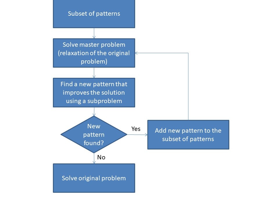
The method starts from a master problem which is a linear relaxation of the original linear programming model (a problem where all variables are real and therefore, there are no integer or binary variables). This problem is solved for a reduced set of variables, columns or, in our example, cutting patterns to determine the minimum number of initial bars and how they must be cut to satisfy the demand and once solved, it is sought if there is any new variable, column or pattern that improves the initial solution (in our case, that manages to reduce the number of initial bars necessary to satisfy the demand) using a subproblem. This iterative process is repeated until no new pattern is found that improves the solution of the master problem, at which point the original problem is solved (an unrelaxed master problem where integer and/or binary variables can exist in addition to real variables) with the initial patterns and with the patterns generated so far.

1. Initial Subset of Patterns

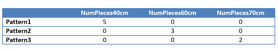
To initialise the method, we are going to use a set of patterns that are easy to generate. In particular, we will use three patterns and in each of them, we will only allow cuts of one type of final product. Thus, pattern 1 indicates that the initial bar will be cut into five 40 cm products, pattern 2 represents that the initial bar will be cut into three 60 cm products and pattern 3 shows that the initial bar will be cut into two 70 cm products.

2. Master Problem

The master problem (linear relaxation of the original programming model where all variables are real) that we are going to use has the following formulation:

The decision variable $(x_p)$ represents the number of initial bars of length 200 cm to be cut by the cutting pattern $p$ and is real type.
There is a constraint that controls that the sum of the final products $f$ (40 cm, 60 cm and 70 cm) cut from each pattern $p$ satisfies the demand.
We have an objective function to minimise the number of initial bars to be used.

Master problem formulation

Indexes:

$p$ $cutting$ $patterns$

$f$ $final$ $products$

Parameters:

$d_f$ $demand$ $for$ $the$ $final$ $product$ $f$

$a_f_p$ $number$ $of$ $final$ $products$ $f$ $in$ $the$ $cutting$ $pattern$ $p$

Variable:

$x_p$ $number$ $of$ $initial$ $bars$ $cut$ $using$ $the$ $cutting$ $pattern$ $p$

Minimise:

$\begin{align*} \sum_{p}x_{p} \end{align*}$

Bound to:

$\begin{align*} \sum_{p} a_{fp}x_{p} \geq d_{f} \hspace{1cm} \forall f\\ x_{p} \geq 0, real \hspace{1cm} \forall p \end{align*}$

3. Sub-problem

The formulation of the sub-problem is as follows:

The decision variable $(y_f)$ corresponds to the number of final products of length $f$ (40 cm, 60 cm or 70 cm) included in the new pattern and is an integer type.
There is a restriction that controls that the sum of the lengths of the products included in the new pattern does not exceed the length of the initial bar.
We have an objective function that maximises the value of the products introduced in the new pattern through the shadow prices of the master problem $(\pi_f)$ . In this case, for a pattern to be finally chosen and become part of the set of patterns that the master problem will work with in the next iteration, a value of the objective function greater than 1 must be reached for that pattern. If this is the case, the reduced cost of the new pattern in the master problem will be negative, which means that the objective function of this problem will be reduced by 1 minus the value of the objective function of the subproblem for each bar that is cut in the master problem using the new pattern, which translates into a saving in the number of bars finally used to cover the demand.

Sub-problem formulation

Indexes:

$f$ $final$ $products$

Parameters:

$\pi_f$ $shadow$ $price$ $associated$ $with$ $the$ $demand$ $constraint$ $f$ $in$ $the$ $master$ $problem$

$w_f$ $length$ $of$ $final$ $product$ $f$

$W$ $initial$ $bar$ $length$

Variable:

$y_f$ $number$ $of$ $final$ $products$ $f$ $included$ $in$ $the$ $cutting$ $pattern$

Maximise:

$\begin{align*} \sum_{f}\pi_{f}y_{f} \end{align*}$

Bound to:

$\begin{align*} \sum_{f} w_{f}y_{f} \leq W \hspace{1cm} \forall f\\ y_{f} \geq 0, integer \hspace{1cm} \forall f \end{align*}$

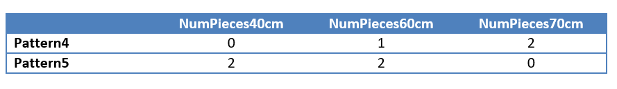
By initialising the method with the three starting patterns, the subproblem has generated the two new patterns shown in the following table, where, for example, pattern 4 proposes to cut the initial bar into one 60 cm and two 70 cm products.

4. Column Generation

Before generating patterns using the decomposition, three patterns were available and the minimum number of bars needed to meet the demand using these patterns is 487.

Using the patterns generated by the decomposition of the originals, five in total, it has been obtained that a total of 410 bars should be purchased and that 60 of them should be cut following pattern 1 (five 40cm products), 200 following pattern 4 (one 60cm product and two 70cm products) and 150 following pattern 5 (two 40cm products and two 60cm products).

This solution exactly meets the demand for end products and is optimal by using as few initial bars as possible and does not generate any waste during the cutting process.

For combinatorial problems such as the one outlined above, the column generation method allows the solution space to be explored quickly and intelligently from a reduced set of starting variables or columns, which makes the running time of this method grow reasonably as the problem size increases.

In this example, the decomposition has only generated two new patterns and the complete problem has only considered five. In a small problem, all possible patterns could be generated without the need for column generation and the problem would work with all of them. However, as long as there were more final products (with different lengths) the number of possible patterns could be extremely high and the problem, with all those patterns, could not be solved in reasonable times. In this case, it is interesting to generate only an initial set and then, through decomposition, add only new potentially interesting patterns.

This method is a sophisticated divide and rule strategy, not included in commercial solvers such as Gurobi, but especially useful not only to solve cutting problems but also complex problems related to shift design, vehicle routing, production scheduling or the planning of site visits by sales or maintenance teams.

1. Initial Subset of Patterns

2. Master Problem

Master problem formulation

Indexes:

Parameters:

Variable:

Minimise:

Bound to:

3. Sub-problem

Sub-problem formulation

Indexes:

Parameters:

Variable:

Maximise:

Bound to:

4. Column Generation

You Might Also Like

Sparklines for Excel

The Astronomical Math Behind UPS’ New Tool to Deliver Packages Faster

School Timetabling