Although prescriptive analytics is not a newcomer, thanks to the attention brought about by big data, machine learning and others, the family’s “older sister” is now much better received. However, due to the lack of knowledge that has existed so far in the industry, there is still some confusion about what to expect and how prescriptive analytics can be used.
In this post we will elaborate on two areas: optimization and simulation, two very powerful tools that allow you to tackle complex problems and make better decisions, always with an impact on the bottom line. But just as the good surgeon knows when to use a scalpel and when to use an X-ray, the expert in advanced analytics must also know when to use optimization and when to use simulation.
Optimization
Optimization consists in the construction of a mathematical model (with variables and equations) whose resolution allows finding the best solution to a problem: the optimal one.
A classic example is the traveling salesman problem (TSP, which we explained here), consisting in visiting a set of cities only once and returning to the city of departure traveling the shortest possible distance.
Optimization has had applications in a very wide range of problems in a multitude of industries. From more conventional cases such as deciding where to locate facilities and with what capacity (supply chain design) to production planning or development of optimal routes for last-mile delivery. There are less known but still very valuable applications such as the movement of sensors that analyse tissues or samples from patient extractions. The sensor has to go through a series of points and the less time it takes to do it (it is a TSP), the greater the number of tests per hour and the sooner it can provide diagnostics.
This YouTube playlist explains the fundamentals of optimization.
Simulation
Simulation consists in building a digital replica (a model) of the system under study with as much detail in each of its elements as required, in such a way that it allows observing the expected behaviour of the system against different configurations. Unlike optimization, it does not automatically offer the best configuration, but it is an ideal tool for the analyst to select configurations, evaluate them, and choose which one to implement.
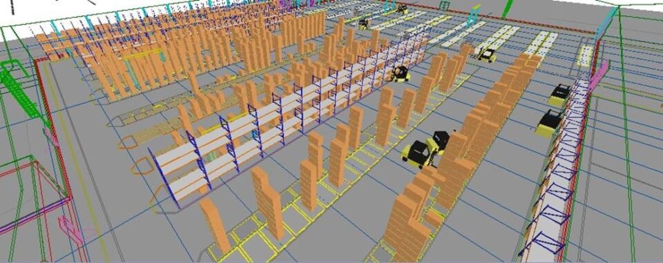
As an example, simulation has been widely used in the redesign of layouts. With a simulation model it is possible to represent in detail where the different sections of a plant are located, their equipment, their process times, the movements of the different parts and batches, the maintenance modules, breakdowns, etc.
Simulation models often incorporate a graphical representation of the system in great detail. It is literally a digital mock-up: we can “see” our system. In the figure above you can appreciate the detail with which a warehouse is represented to evaluate different layouts, which corresponds to a model developed in Simio. There are different ways of storing boxes, trolleys, and the aisles through which they circulate, for example.
We can do different analyses using this model. For example, evaluate different ways of locating references and quantifying their impact on productivity; the number of trucks can be changed; we can compare different alternatives for picking… We can study any potentially interesting action in a short time, without risk and at a very low cost, with the confidence that we know what will happen in our warehouse when we implement what we have previously studied in our model.
Why simulation?
It is worth asking why resort to simulation when optimization can provide “the optimum”, that is, why delegate to the analyst the work of exploring alternatives using a simulation model when an optimization model provides the best solution.
Optimization models must be solved in a reasonable time and for this, in many cases, the system cannot be represented in all detail. For example, determining the sequence with which models are introduced into an assembly line in the context of car manufacturing can be done with optimization, because the operating times at each station on the line are well known. However, in other contexts this may not be the case, and tasks may have a variable unknown duration (for example, between 10 and 20 minutes). Representing this time variability in detail would make an optimization model ineffective (we would not find a solution to implement it in time).
The same happens with the times between failures, the duration of repairs, the possibility that a process cannot be carried out due to a lack of raw material, the unavailability of resources (including human resources) due to some type of incident … It is not possible to introduce all that detail in an optimization model and therefore we might consider working with average values.
The question then is, why not work with average values? Let’s see it with an example.
Simulation example: the case of Bob and Ray
The case of Bob and Ray (Jacobs, 2011) illustrates this simply. Bob and Ray work on a small assembly line. Bob begins assembling the product for which he performs a series of operations and when he finishes he passes it on to Ray who continues with another set of operations. Once a product has had the operations carried out by Bob and those carried out by Ray, we have a finished product.
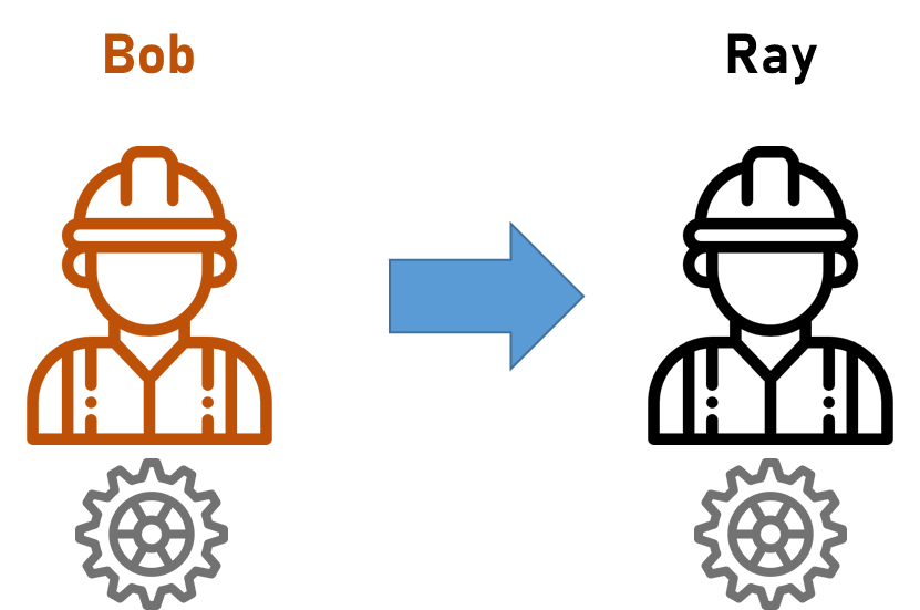
There is no room to store products between Bob and Ray. So if Ray hasn’t finished assembling a product and Bob has, Bob is stuck until Ray finishes. Likewise, if Ray is finished and Bob is not, Ray must wait until Ray is finished and delivers the product to him to continue working.
Lastly, Bob and Ray don’t always take the same amount of time in their respective operations. They can take between 10 and 80 seconds. As shown in the table below, Bob takes 10 seconds 4% of the time, 20 seconds 6%, and so on.
| Seconds | Bob | Ray |
|---|---|---|
| 10 | 4% | 8% |
| 20 | 6% | 10% |
| 30 | 10% | 12% |
| 40 | 20% | 14% |
| 50 | 40% | 20% |
| 60 | 11% | 16% |
| 70 | 5% | 12% |
| 80 | 4% | 8% |
It’s easy to see that Bob, on average, takes 45.9 seconds per product and Ray 46.4, a little slower. If we worked with average values, we could expect Ray to set the pace because he is the slowest, an assembled product would be obtained every 46.6 seconds and Ray would be working all the time while Bob would hardly rest, 0.5 seconds (46.4-45.9) per product.
However, this analysis does not take into account that sometimes Bob will take close to 80 and Ray close to 10 seconds, so Ray will be idle and, conversely, Ray will sometimes be the one who uses a high time and Bob a low time, so Bob will be blocked. Since there is no buffer, the production capacity is less than if Bob and Ray always took the same average time.
This playlist introduces the fundamentals of simulation, and in particular this example in more detail, and shows a simulation model in its most elementary version that allows estimating the actual occupancy levels for Bob and Ray.
Why optimization?
So, we have another question, why do we want to use optimization models then?
Optimization models are especially desirable when information is admitted to be known, in which case the models will prescribe the optimum. Optimization models also allow for the explicit incorporation of uncertainty (through robust optimization, stochastic optimization, etc.)
However, sometimes the detail required by analysis and the uncertainty of the data make the optimization-only approach not sufficient.
In these cases, a somewhat simplified optimization model can be developed with deterministic information (mean times, for example). A simulation model can then be used to evaluate with all realism the impact on the solution suggested by the optimization model and explore alternatives around it.
The line balancing problem lends itself to effective cooperation between optimization and simulation. This playlist presents the problem and how a solution can be obtained by means of optimization and average values.
This playlist then presents a simulation model to assess the impact of uncertainty and what performance can be expected from the assembly line when configured according to the optimization model, also taking uncertainty into account.
Last, Borreguero (2020) presents an analogous example in the airframe manufacturing sector. On the one hand, an optimization model is developed to obtain production planning without taking into account failures in supplier deliveries, variability of process times, rework due to execution errors, absenteeism, etc. The solution obtained from the optimization model is introduced into a simulation model that does incorporate all these sources of uncertainty and, with this, it is possible to assess whether demand can really be met with the production plan obtained. Should that not be the case, the same simulation model is used to explore similar solutions that do allow us to serve it.
Conclusion
To summarize, good surgeons have a good knowledge of all the instruments at their disposal and when to use each. Optimization and simulation are very valuable techniques and there are certain cases in which the combination of the two can deliver even more value. There are other tools, such as forecasting techniques that can be combined with the above. For example, a forecast model may help reduce uncertainty and feed more reliable data into our simulation and optimization models. This topic will be covered in another post.
References
Jacobs, F. Robert, Richard B. Chase, and Rhonda R. Lummus. Operations and supply chain management. Vol. 567. New York: McGraw-Hill Irwin, 2011.
Borreguero Sanchidrián, Tamara. Scheduling with limited resources along the aeronautical supply chain: from parts manufacturing plants to final assembly lines. Diss. Universidad Politécnica de Madrid, 2020.
Authors
Dr. Tamara Borreguero holds a PhD in industrial engineering (UPM) and currently is an Expert in line balancing and scheduling in Airbus Defence and Space.
Dr. Álvaro García holds a PhD in industrial engineering (UPM), works as a professor at UPM and is a co-founder at baobab soluciones.
