
Improving the allocation of ambulances to their bases in a city, so that they cover the entire area and serve all residents in the best possible way, implies a shorter reaction time to an emergency with the same resources, which directly benefits everybody’s well-being. The situations where an ambulance may be needed are potentially life-threatening. Dimensioning an ambulance service is a problem for which it is worth using mathematics to find the best possible solution.
It is not an easy problem to solve. Using metrics based on means or old data is misleading, especially if there are not enough records. Approaches based on k-means or coverage models are poor. On average an ambulance can have good intervention times, but if all the ambulances in a base are busy, times extend beyond acceptable.
Therefore, as part of our knowledge generation initiatives, we have proposed and developed a novel methodology based on Simulated Annealing and simulations.
Broadly speaking, the method consists in the following:
- Create an initial solution using a simple algorithm and thereby establish how many ambulances there are initially in each base
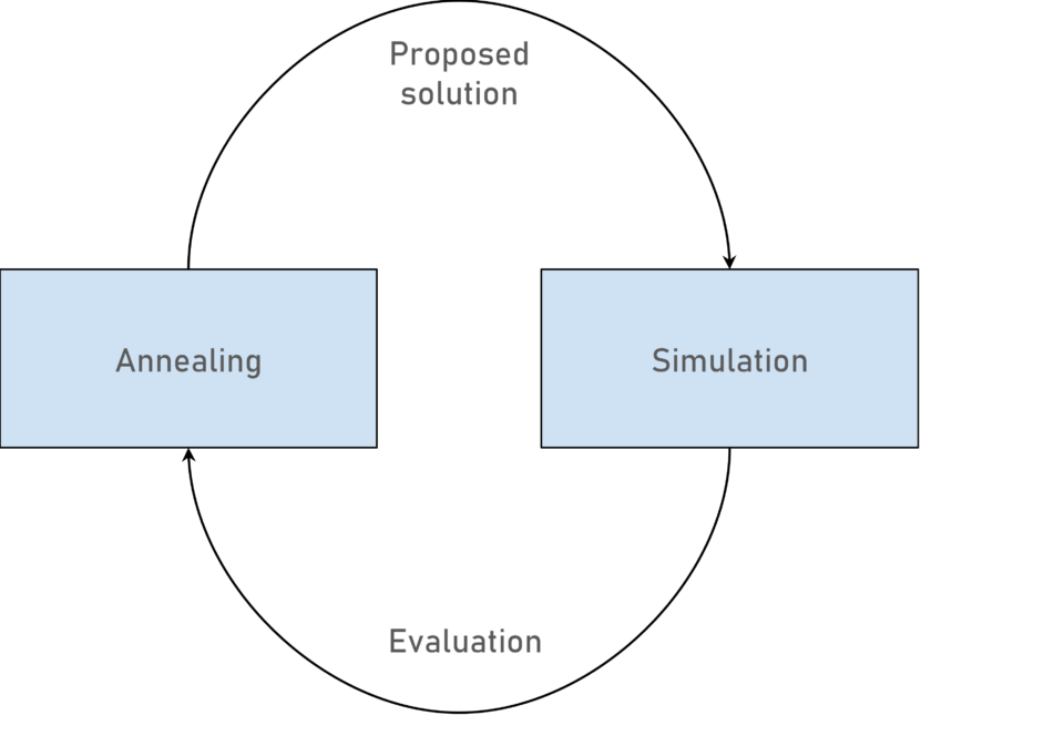
- Evaluate the solution not by means of an analytical expression but by using a simulation model to characterise what the expected operation would be in reality. The model will return an indicator of the suitability of the solution, which we will call energy and which should be as low as possible.
- Collect the simulation information. Depending on the result, the evaluated solution is discarded or accepted as a new current solution. This current solution will be used to create a new solution.
- Repeat steps 2 and 3 and keep the best solution.
Simulated Annealing
Simulated Annealing is a metaheuristic search algorithm for optimisation problems. This means that instead of systematically calculating the optimal solution to a problem, it explores the solution space using certain assumptions until a good enough solution is found. The typical justification for this approach is the lack of calculation capacity.
The name ‘simulated annealing’ is inspired by the metallurgical annealing technique, which consists of controlled heating and cooling of a material to increase the dimensions of its crystals and eliminate its defects.
In this case we apply the following process.
- Starting off an initial solution obtained in a simple, even random way (random assignment of ambulances to bases), we simulate the energy of the solution. In all probability this energy will be high.
- We make a slight change in the initial solution (we reallocate an ambulance to another base), calculate the energy of this new solution and compare it to the previous one.
- If the energy difference is negative, that is, the new solution is better than the previous one, we discard the previous solution, keep the new one and repeat the previous step.
- If the energy difference is positive, that is, the new solution is worse than the previous one, in order to escape local optima we can still keep the new solution if the energy difference is small. In order to do this, we calculate a factor p between 0 and 1, which decreases with the energy difference and increases with another parameter that we will call temperature, and then generate a random number between 0 and 1. If this number is less than p, we will accept the new solution.
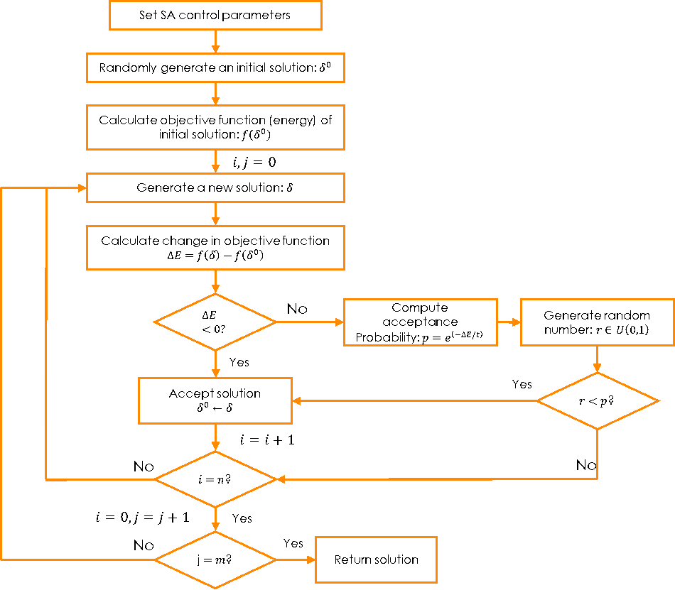
This process is embedded in two loops that determine how long it runs. An inner loop counts how many solutions are calculated for each temperature. An external loop counts how many temperature values will be considered, from highest to lowest. In other words, we will reduce the algorithm temperature a predefined number of occasions.
Simulation
The objective of the simulation is to measure the suitability of each base allocation plan (the solutions). It generates fictitious emergencies in different locations in the analysed area, calculates the distance from each of the available vehicles and assigns the closest vehicle; if necessary, it considers the time and distance the vehicle would spend heading to the hospital and returning to its base. The simulation considers that the vehicle is already available to attend another emergency on the way back to base.
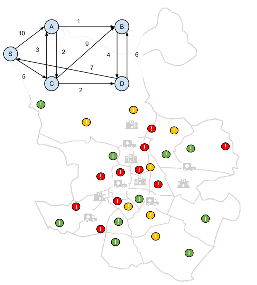
To facilitate development and reduce computation times, the simulation divides the city into zones and defines a node for each zone, to which it will assign all emergencies generated in said zone. In this way, the city is represented as a mosaic of zones and a network of interconnected nodes. Thus travel times between each node and its adjacent nodes can be determined using public APIs and it is possible to apply Dijkstra’s algorithm to calculate the shortest path between any two nodes.
Results
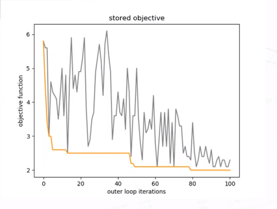
This method allows to tackle a difficult problem with traditional methods. The graphs below show how temperature changes and how the probability of accepting a new solution evolve in a problem execution with 100 temperature values (external loop) and 20 iterations for each value (internal loop).
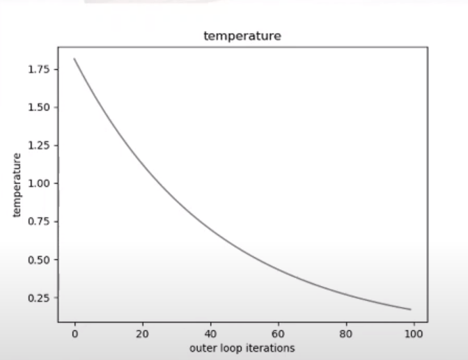
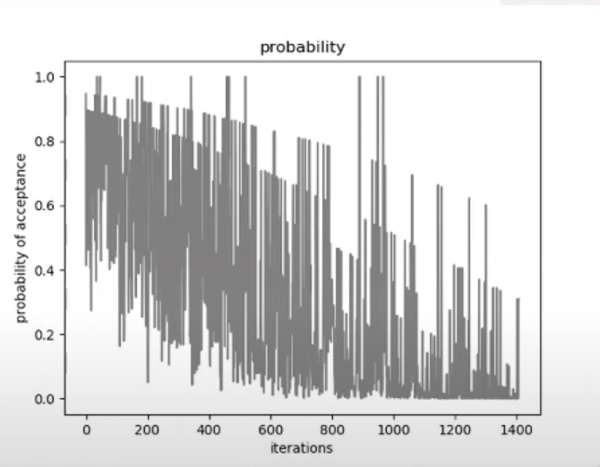
The lower graph clearly shows how the energy of the best solution found for each temperature decreases and how the algorithm is allowed to explore worse solutions in order to access others that offer a better result (sometimes to reach the highest top you need to cross a valley).